Introduction
In this post, I’m going to make the claim that we can simplify some parts of the machine learning process by using the analogy of making soup. I think this analogy can improve how a data scientist explains machine learning to a broad audience, and it provides a helpful framework throughout the model building process.
Relying on some insight from the CRISP-DM framework, my own experience as an amateur chef, and the well-known iris data set, I’m going to explain why I think that the soup making and machine learning connection is a pretty decent first approximation you could use to understand the machine learning process.
This post is pretty light on code, with just a few code chunks for illustrative purposes. These are the packages we’ll need.
library(tidyverse)
library(glmnet)
library(caret) # caret or carrot? :)
The code for this post can be found on my GitHub.
Some Background

The CRISP-DM Framework (Kenneth Jensen) CC BY-SA 3.0, Link
I recently gave a presentation on the CRISP-DM framework to the various teams that make up the IT Department at my organization. While I was discussing the Modeling phase of CRISP-DM, I got some questions that come up when you talk about data science with software-minded audiences.
When you’re building a model, what are you doing? Where are you spending your time? How long does that take?
The people in IT know that data, machine learning, and artificial intelligence are impacting their daily lives, from chat bots to spam email detection to the curation of news feeds. While they have awareness of the impact of data science, they may not have as much awareness of the processes of data science. I think the responsibility of demystifying machine learning rests on data scientists, and it’s imperative to have comprehensible mental models that can be employed to describe and de-clutter the machine learning process.
In my response to the questions, I thought I did a fairly good job of breaking down the three components of machine learning and the typical amount of iteration within each component by mirroring the CRISP-DM breakdown:
- Problem type and associated modeling technique
- Iteration level: low
- Parameter tuning
- Iteration level: high
- Feature engineering and selection
- Iteration level: high
Of course, I was in a room full of very smart people, trying to extemporaneously explain parameter tuning and feature engineering in a coherent way, so I probably could have done a better job.
A few minutes after the meeting, I realized I could have used a simple analogy to explain the machine learning process.
Machine learning is like making a soup. First, you pick the type of soup you want to make. Second, you figure out the ingredients that are going to be in the soup and how they should be prepared. Third, you determine how you’re going to cook the soup. Finally, you taste the soup and iterate to make it taste better.
Making a Soup = Machine Learning
While I’m certainly not an expert chef, I think you can boil down making a soup into a few simple components.
Picking the Soup = Selecting a Modeling Technique
In this step, we’re just trying to figure out what we want to make. In the machine learning world, this is where we need to think carefully about the problem we’re trying to solve, and which of the many machine learning algorithms can be used to attack it.
Soup Making: what type of soup are we trying to make? are there external characteristics (season, weather, mood) we should consider? what soup will we enjoy? how difficult is this soup to make?
Machine Learning: what type of question(s) are we trying to answer? what type of model will allow us to answer this question? how is this model implemented? what are its assumptions?
Ingredients = Feature Engineering & Selection
Now that we’ve decided what we’re going to make, we need to head to the grocery store and pick up the ingredients. After that we’ll need to prepare the ingredients for cooking. Similarly, we’ll need to understand the variables and context for our data set, and create/transform/aggregate our variables to get them into a useful form for modeling.
Soup Making: what vegetables are needed and how should they be prepped? what type of protein will we be using? do we need some type of stock for the soup?
Machine Learning: what variables are needed for this model? do we need to standardize any of the variables? are there non-numeric variables? if so, how should those be handled?
Cooking Methods = Parameter Tuning
Once we’ve decided upon the type of soup and the ingredient, it comes time to make the soup. This step involves select the best combination of different cooking methods to make the optimal (i.e. most tasty) soup. When we perform parameter tuning, we’re trying to pick the best combination of values to make our machine learning algorithms reach optimal performance. These values are different from the variables we previously discussed, as the variables are the inputs for our ML algorithms, while the tuning parameters describe the algorithm itself.
Soup Making: what heat are we cooking at and for how long? is the pot covered or uncovered? will the pot be on the stove top for the entirety of cooking or will we move it to the oven? how long will we let the soup simmer? how big of a batch are we making?
Machine Learning: what is our loss function? is there a learning rate? what’s the k in our k-fold cross validation? how many trees in our random forest? how much should we penalize complexity? what is the training/validation split? does an ensemble model outperform a single model?
Building a Model
Let’s see this framework in action. I’m going to pick a straightforward classification task to demonstrate. I’m going to use the iris dataset and try to predict whether a flower is from the setosa species.
Here’s a quick look at the data:
| Sepal.Length | Sepal.Width | Petal.Length | Petal.Width | Species |
|---|---|---|---|---|
| 5.1 | 2.5 | 3.0 | 1.1 | versicolor |
| 6.0 | 2.2 | 5.0 | 1.5 | virginica |
| 5.1 | 3.5 | 1.4 | 0.2 | setosa |
| 6.6 | 3.0 | 4.4 | 1.4 | versicolor |
| 4.9 | 2.5 | 4.5 | 1.7 | virginica |
| 6.3 | 3.3 | 4.7 | 1.6 | versicolor |
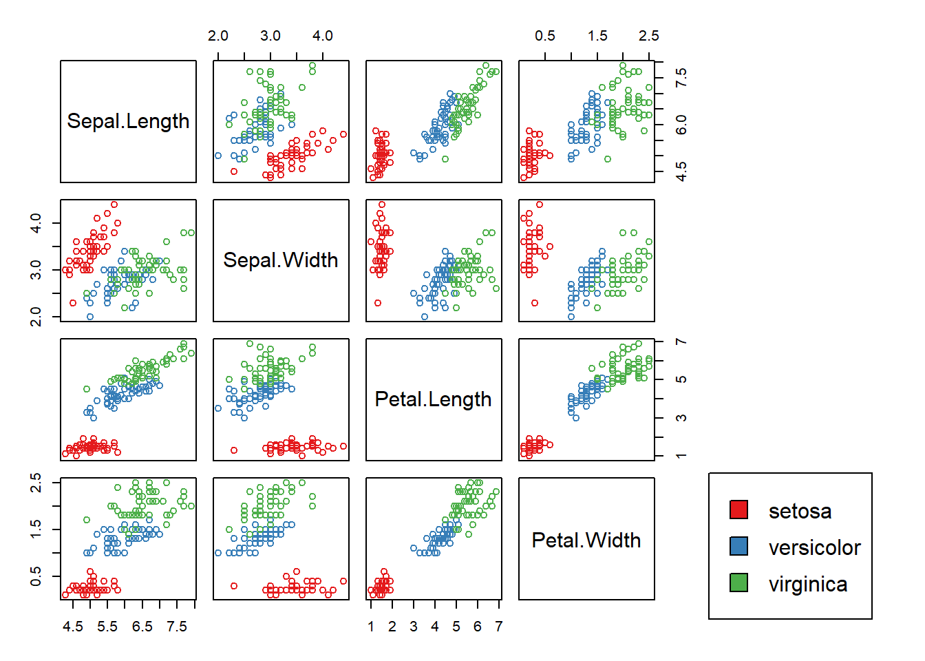
Just looking at the scatterplot matrix above, we can see that trying to classify flowers into the setosa species is a bit of a toy problem (the red points are well-separated from the blue and green). In fact, just by examining if the petal length of a flower is smaller than 2.45, we can determine if the flower is from the setosa species.
table('Petal Cut' = iris$Petal.Length >= 2.45,'Setosa' = iris$Species == 'setosa')## Setosa
## Petal Cut FALSE TRUE
## FALSE 0 50
## TRUE 100 0The iris data is used as a “hello, world” in data science. It has nice applications across a broad spectrum of applications: clustering, regression, classification, and visualization. It’s worth getting excited about!
Picking the Soup
As discussed earlier, the problem we’re trying to tackle is predicting if a flower is from the setosa species. Since we already know that there is something we’re trying to predict, we only have to explore supervised machine learning algorithms. We also know that we’re not interested in building a model which generates predictions on a continuous range. We only want the answer a binary question: is this a setosa or not?
This narrows the set of algorithms even further, and we only need to explore models which will either generate a classification for a flower, or will generate a probability of the flower’s species being setosa.
For this post, I’m going to use elastic net logistic regression. Elastic net fits a logistic regression while also penalizing the complexity of the model. The excellent glmnet package allows us to build models in this fashion. I’m going to use ridge regression (elastic net with \(\alpha=0\)), which penalizes the \(L_2\) norm of the coefficients. Fitting an elastic net with \(\alpha=1\) generates a LASSO model, which can also be useful for variable selection, but I’m using a different technique to do variable selection in this post, so I’m sticking with ridge here.
Ingredients
Feature engineering and selection is one of the most time-consuming parts of the machine learning process. To keep this post brief, I’m going to go through just a few feature engineering steps.
First, we split the data into training and testing sets. After this, I extract only the numeric predictor variables for the model, and then add squared terms as well as interactions between each of the first order effects. These two steps transform the predictor matrix from four columns into fourteen. Finally, we use the preProcess function from the caret package to center and scale each variable so that it has mean = 0 and variance = 1.
set.seed(123)
# create training and testing split
training_index <- sample(nrow(iris), 0.7 * nrow(iris))
iris_train <- iris[training_index,]
iris_test <- iris[-training_index,]
# grab X data add squared term for each column
iris_X_train <- iris_train[,-5] %>% mutate_all(funs('sq' = . ^ 2))
iris_X_test <- iris_test[,-5] %>% mutate_all(funs('sq' = . ^ 2))
# all two way interactions with first order terms
iris_X_train <-
  model.matrix(~-1 + . + (Sepal.Length+Sepal.Width+Petal.Length+Petal.Width) ^ 2,
               data = iris_X_train)
iris_X_test <-
  model.matrix(~-1 + . + (Sepal.Length+Sepal.Width+Petal.Length+Petal.Width) ^ 2,
               data = iris_X_test)
# fit center and scale processor on training data
preProc <- preProcess(iris_X_train)
iris_X_train_cs <- predict(preProc, iris_X_train)
iris_X_test_cs <- predict(preProc, iris_X_test)
# labels, convert to factor for glmnet
iris_y_train <- as.factor(as.numeric(iris_train$Species == 'setosa'))
iris_y_test <- as.factor(iris_test$Species == 'setosa')
The data augmentation steps I went through created numeric variables, but we could use decision trees or similar techniques to create categorical variables from numeric. We use those methods when it’s unnecessary to retain the continuous nature of a numeric variable (often the case with age or physiological measurements like height or weight).
After we’ve gone through the feature engineering step, we can think about which variables we’ll actually want to use in our model. There can be considerable back-and-forth between feature engineering and feature selection, just like iterating on a recipe may involve different ingredients and different ways of preparing those ingredients.
To do feature selection, I’m going to once again turn to the caret package and use the rfe function. We could also use the infrastructure of the glmnet package to do some feature selection, as the LASSO helps us perform variable selection.
set.seed(123)
rf_control <- rfeControl(rfFuncs, method = 'cv', number = 5)

iris_rfe <- rfe(x = iris_X_train_cs,
                y = iris_y_train,
                sizes = 2:14, # select at least two variables
                rfeControl = rf_control)

iris_rfe$optVariables
## [1] "Petal.Length:Petal.Width" "Sepal.Length:Petal.Width"The procedure we used for variable selection suggested an interaction between the petal length and petal width variables, and petal length squared. It’s usually a bad idea to include higher ordered terms without also including the lower order terms, so our final model will have three variables: petal width, petal length, and petal width * petal length interaction.
Cooking Methods
In elastic net regression, we have two parameters to select: \(\alpha\) and \(\lambda\). \(\alpha\) controls the weight we give to the \(L_1\) and \(L_2\) penalties (with \(\alpha\) being placed on the \(L_1\) norm, and \(1-\alpha\) being placed on the \(L_2\) norm). Putting all the weight on \(L_2\) norm is better known as Tikhonov regularization or ridge regression. I’ve already made my choice of \(\alpha\) for this post, so we don’t have to tune it.
The other parameter we need to tune is \(\lambda\), which controls the strength of the penalty we’ll place on the \(L_2\) norm of the coefficients. A higher \(\lambda\) value will “shrink” the model’s coefficients, whereas a smaller \(\lambda\) value will result in a model more similar to the standard unregularized logistic regression fit.
The cv.glmnet function allows us to use cross-validation to tune \(\lambda\).
vv <- c("Petal.Width", "Petal.Length", "Petal.Length:Petal.Width")

iris_X_train_cs_sub <- iris_X_train_cs[, colnames(iris_X_train_cs) %in% vv]
iris_X_test_cs_sub <- iris_X_test_cs[, colnames(iris_X_test_cs) %in% vv]
cv_glm1 <- cv.glmnet(x = iris_X_train_cs_sub, y = iris_y_train,
alpha = 0, family = 'binomial',
nfolds = length(iris_y_train) - 1,# LOOCV
standardize = FALSE, intercept = FALSE)
lambda_1se_1 <- cv_glm1$lambda.1se # store "best" lambda for now
plot(cv_glm1)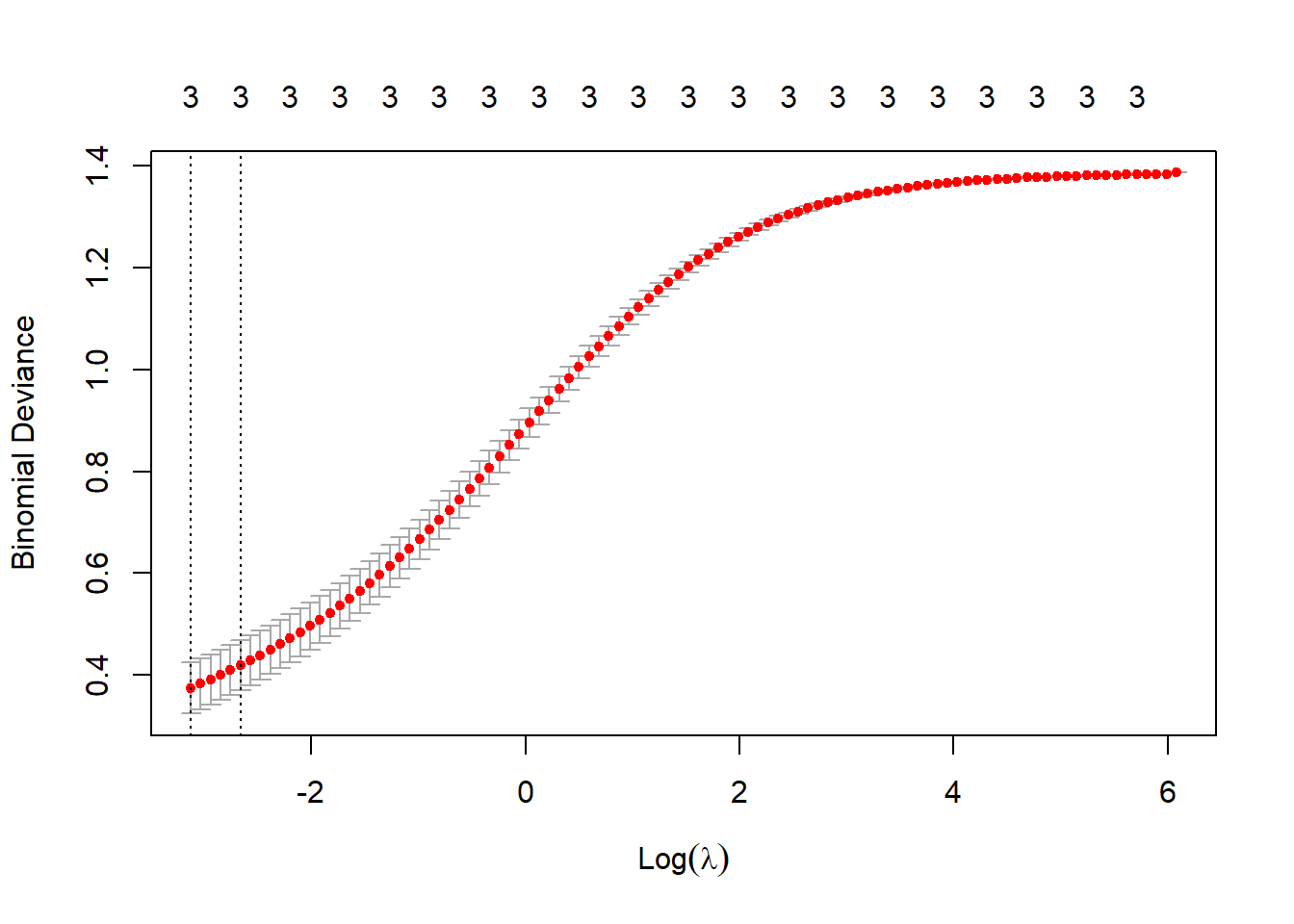
We can explore \(\lambda\) a bit more to improve the model fit.
cv_glm2 <- cv.glmnet(x = iris_X_train_cs_sub, y = iris_y_train,
                     alpha = 0, lambda = exp(seq(-10, log(lambda_1se_1), length.out = 500)),
                     family = 'binomial', nfolds = length(iris_y_train) - 1,# LOOCV
                     standardize = FALSE, intercept = FALSE)

lambda_2 <- exp(-6.5)
plot(cv_glm2)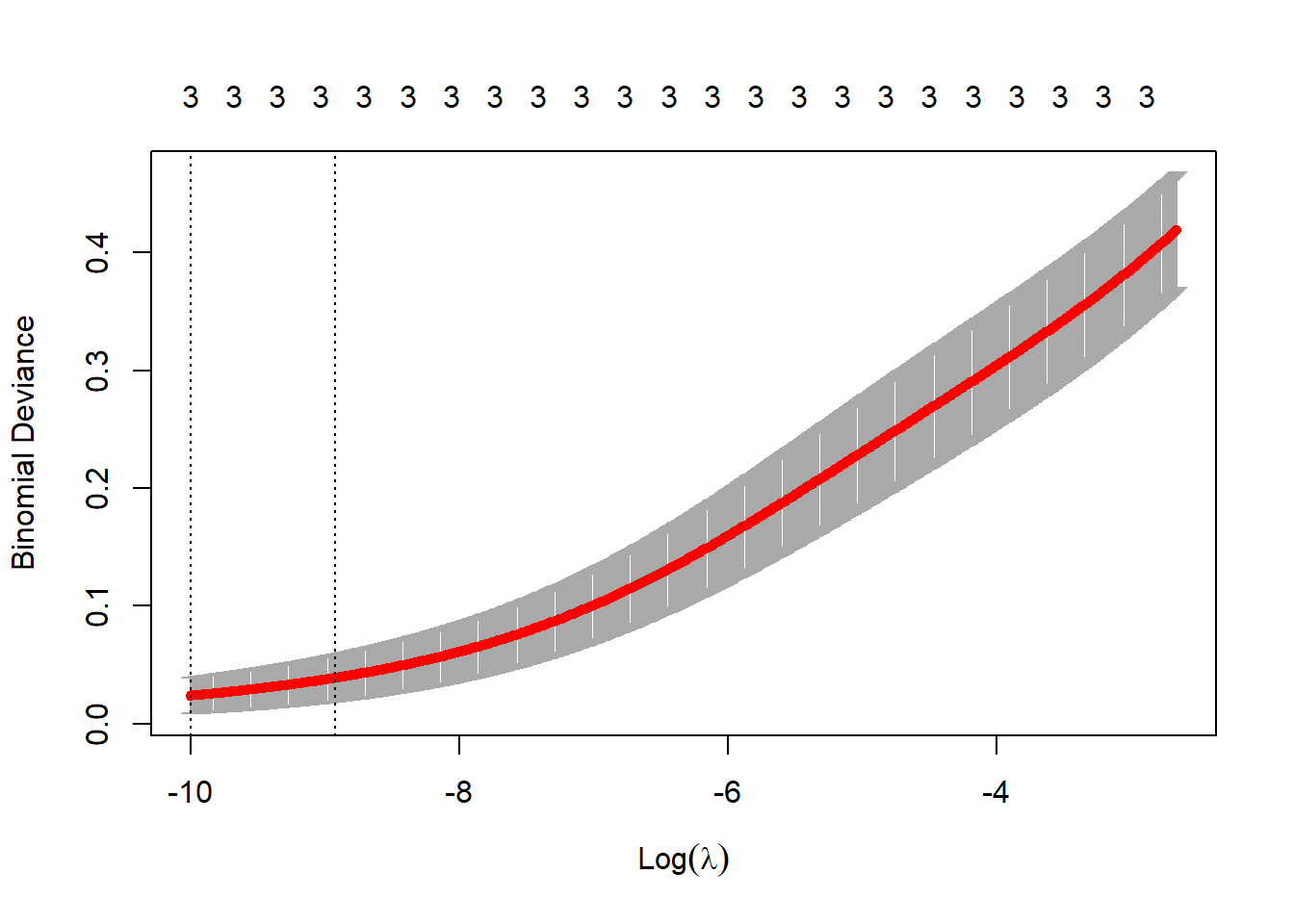
Cross-validation suggests a rather small value of \(\lambda\), indicating that the model’s fit doesn’t improve with a high degree of regularization. In the next section, we’ll use two values of \(\lambda\) to fit the model (\(\lambda_1\) = 0.0698, \(\lambda_2\) = 0.0015), and then investigate the results.
Tasting the soup
After we fit the model (or make the soup), we have to determine how good it is. For this example, I’m going to use a simple method for determining the classification accuracy and check the % of time the classifier got the species correct. Using this metric implies that we’re treating false positive and false negatives as equally bad errors. In most real world situations, this is not the case.
# naive classification accuracy
class_acc <- function(preds, labels, thresh = 0.5){
  tt <- table(preds > thresh, labels)
  sum(diag(tt)) / sum(tt)
}
In addition to the two models fit using regularization, I’m going to fit an unregularized model with the selected features along with an unregularized model with only the variables that were present in the original dataset.
# regularized models
ridge_1 <- glmnet(x = iris_X_train_cs_sub, y = iris_y_train,
                  family = 'binomial', lambda = lambda_1se_1, alpha = 0,
                  standardize = FALSE, intercept = FALSE)
ridge_2 <- glmnet(x = iris_X_train_cs_sub, y = iris_y_train,
                  family = 'binomial', lambda = lambda_2, alpha = 0,
                  standardize = FALSE, intercept = FALSE)
# unregularized
glm1 <- glm(iris_y_train ~ -1 + ., data = data.frame(iris_X_train_cs_sub),
            family = 'binomial')
glm2 <- glm(iris_y_train ~ -1 + Sepal.Length+Sepal.Width+Petal.Length+Petal.Width,
            data = data.frame(iris_X_train_cs),
family = 'binomial') | model | type | class accuracy |
|---|---|---|
| ridge_1 | regularized-lambda1 | 84.4% |
| ridge_2 | regularized-lambda2 | 95.6% |
| glm1 | full | 100.0% |
| glm2 | original | 100.0% |
In the table above, we can see that the unregularized models resulted in better predictions on our test set. This shouldn’t be too surprising, as this classification example is somewhat contrived. In more realistic settings, we may see better predictive performance from models fit using regularization.
Wrapping Up
When we compare making a soup to machine learning, we get a simple and understandable lens through which we can look at machine learning. Just like making soup or cooking in general, iteration is a key component of machine learning. If you ask anyone that’s trying to develop a recipe, they probably won’t get it right the first time. If they do get it right the first time, maybe that’s because
- they got lucky
- they aren’t trying to make too difficult of a dish
- they’re an experienced cook
These situations have clear parallels to machine learning. Maybe you got lucky and your prediction task is fairly easy or maybe all you need is a simple model or maybe you’re an experienced data scientist.
I feel like this analogy is a pretty straightforward way to explain machine learning to a broad audience of people that are interested in the topic. I found a similar article which discussed ideas that are related to the ones I talked about in my post. If you know of any other posts with similar sentiments, I hope you’ll share them with me!
Thanks for reading my post and leave a comment below if you have any thoughts or feedback!