One of my favorite data science blogs comes from James McCaffrey, a software engineer and researcher at Microsoft. He recently wrote a blog post on a method for allocating turns in a multi-armed bandit problem.
I really liked his post, and decided to take a look at the algorithm he described and code up a function to do the simulation in R.
Note: this is strictly an implementation of Dr. McCaffrey’s ideas from his blog post, and should not be taken as my own.
You can find the .Rmd file for this post on my GitHub.
Background
The basic idea of a multi-armed bandit is that you have a fixed number of resources (e.g. money at a casino) and you have a number of competing places where you can allocate those resources (e.g. four slot machines at the casino). These allocations occur sequentially, so in the casino example, we choose a slot machine, observe the success or failure from our play, and then make the next allocation decision. Since we’re data scientists at a casino, hopefully we’re using the information we’re gathering to make better gambling decisions (is that an oxymoron?).
We want to choose the best place to allocate our resources, and maximize our reward for each allocation. However, we should shy away from a greedy strategy (just play the winner), because it doesn’t allow us to explore our other options.
There are different strategies for choosing where to allocate your next resource. One of the more popular choices is Thompson sampling, which usually involves sampling from a Beta distribution, and using the results of that sampling to determine your next allocation (out of scope for this blog post!).
Code: roulette_wheel
The following function implements the roulette wheel allocation, for a flexible number of slot machines.
The function starts by generating a warm start with the data. We need to gather information about our different slot machines, so we allocate a small number of resources to each one to collect information. After we do this, we start the real allocation. We pick a winner based on how its cumulative probability compares to a draw from a random uniform distribution.
So, if our observed success probabilities are
| machine | observed_prob | cumulative_prob | selection_range |
|---|---|---|---|
| 1 | 0.2 | 0.2 | 0.0-0.2 |
| 2 | 0.3 | 0.5 | 0.2-0.5 |
| 3 | 0.5 | 1.0 | 0.5-1.0 |
And our draw from the random uniform was 0.7, we’d pick the third arm (0.7 falls between 0.5 and 1). This selection criteria is the main point of Dr. McCaffrey’s algorithm. For a better and more thorough explanation, I’d suggest reading his blog post.
We then continue this process (playing a slot machine, observing the outcome, recalculating observed probabilities, and picking the next slot machine) until we run out of coins.
And here’s the code
roulette_wheel <- function(coins = 40,
                           starts = 5,
                           true_prob = c(0.3, 0.5, 0.7)){
  # must have enough coins to generate initial empirical distribution
  if (coins < (length(true_prob) * starts)){
    stop("To generate a starting distribution, each machine must be",
         " played ",
         starts,
         " times - not enough coins to do so.")
  }
  # allocate first ("warm up")
  SS <- sapply(true_prob, FUN = function(x) sum(rbinom(starts, 1, x)))
  FF <- starts - SS
  # calculate metrics used for play allocation
  probs <- SS / (SS + FF)
  probs_normalized <- probs / sum(probs)
  cumu_probs_normalized <- cumsum(probs_normalized)
  # update number of coins
  coins <- coins - (length(true_prob) * starts)
  # create simulation data.frame
  sim_df <- data.frame(machine = seq_along(true_prob),
                       true_probabilities = true_prob,
                       observed_probs = probs,
                       successes = SS,
                       failures = FF,
                       plays = SS + FF,
                       machine_played = NA,
                       coins_left = coins)
  # initialize before while loop
  sim_list <- vector('list', length = coins)
  i <- 1
  # play until we run out of original coins
  while(coins > 0){
    # which machine to play?
    update_index <- findInterval(runif(1), c(0, cumu_probs_normalized))
    # play machine
    flip <- rbinom(1, 1, true_prob[update_index])
    # update successes and failure for machine that was played
    SS[update_index] <- SS[update_index] + flip
    FF[update_index] <- FF[update_index] + (1-flip)
    # update metrics used for play allocation
    probs <- SS / (SS + FF)
    probs_normalized <- probs / sum(probs)
    cumu_probs_normalized <- cumsum(probs_normalized)
    # update number of coins
    coins <- coins - 1
    # update simulation data.frame (very inefficient)
    sim_list[[i]] <- data.frame(machine = seq_along(true_prob),
                                true_probabilities = true_prob,
                                observed_probs = probs,
                                successes = SS,
                                failures = FF,
                                plays = SS + FF,
                                machine_played = seq_along(true_prob) == update_index,
                                coins_left = coins)
    i <- i + 1
  }
  # show success:failure ratio
  message("Success to failure ratio was ",
          round(sum(SS) / sum(FF), 2),
          "\n",
          paste0("(",
                 paste0(SS, collapse = "+"),
                 ")/(",
                 paste0(FF, collapse = "+"), ")"))
  # return data frame of values from experiment
  rbind(sim_df, do.call('rbind', sim_list))
}
Data Analysis
I’ll show a brief example of what we can do with the data generated from this function.
set.seed(123)
rw1 <- roulette_wheel(coins = 5000,
starts = 10,
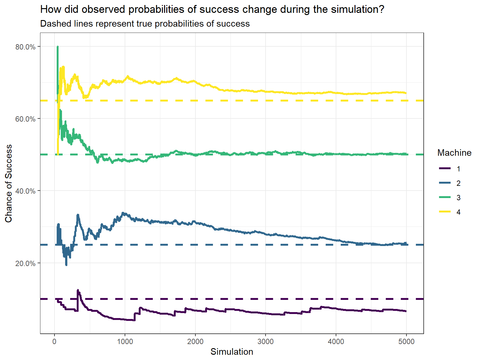
true_prob = c(0.1, 0.25, 0.5, 0.65))## Success to failure ratio was 1.06
## (15+228+835+1490)/(213+662+826+731)| machine | true_probabilities | observed_probs | successes | failures | plays | machine_played | coins_left |
|---|---|---|---|---|---|---|---|
| 1 | 0.10 | 0.0658 | 15 | 213 | 228 | FALSE | 0 |
| 2 | 0.25 | 0.2562 | 228 | 662 | 890 | FALSE | 0 |
| 3 | 0.50 | 0.5027 | 835 | 826 | 1661 | FALSE | 0 |
| 4 | 0.65 | 0.6709 | 1490 | 731 | 2221 | TRUE | 0 |
Let’s look at how the observed probabilities changed over time:
And how did our plays for each machine accumulate through time?
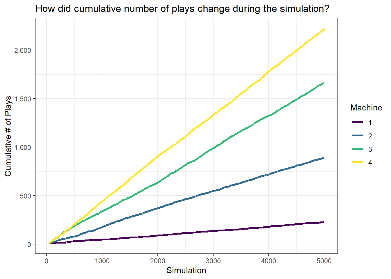
Boring!
Maybe if we run a smaller number of simulations, we might get a better sense of variation in our number of plays.
set.seed(1)
rw2 <- roulette_wheel(coins = 100,
                      starts = 5,
                      true_prob = c(0.1, 0.3, 0.65))
## Success to failure ratio was 0.82
## (1+16+28)/(11+26+18)| machine | true_probabilities | observed_probs | successes | failures | plays | machine_played | coins_left |
|---|---|---|---|---|---|---|---|
| 1 | 0.10 | 0.0833 | 1 | 11 | 12 | FALSE | 0 |
| 2 | 0.30 | 0.3810 | 16 | 26 | 42 | FALSE | 0 |
| 3 | 0.65 | 0.6087 | 28 | 18 | 46 | TRUE | 0 |
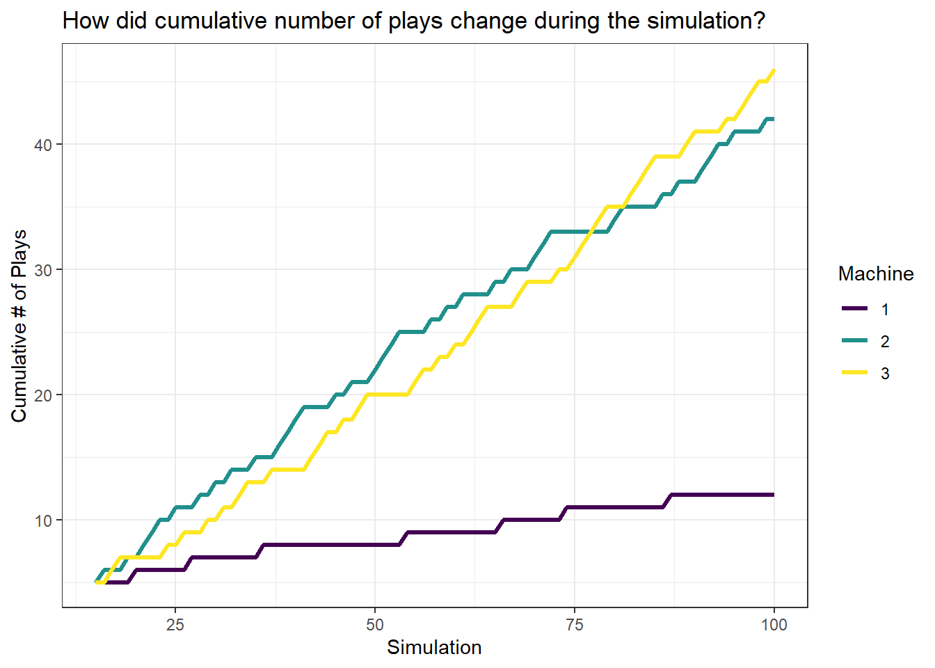
That shows our allocations a little bit better than the previous visualization.
Conclusion
This was a fun exercise for me, and it reminded me of a presentation I did in graduate school about a very similar topic. I also wrote a roulette wheel function in Python, and was moderately successful at that (it runs faster than my R function, but I’m less confident in how “pythonic” it is).
My biggest concern with this implementation is the potential situation in which our warm start results in all failures for a given slot machine. If the machine fails across the warm start, it will not be selected for the rest of the simulation. To offset this, you could add a little “jitter” (technical term: epsilon) to the observed probabilities at each iteration. Another option would be to generate a second random uniform variable, and if that value is very small, you that pull a random lever, rather than the one determined by the simulation.
Finally, I’d be interested in comparing the statistical properties of this algorithm and others that are used in sequential allocation problems…if I have the time.