Recommendation engines have a huge impact on our online lives. The content we watch on Netflix, the products we purchase on Amazon, and even the homes we buy are all served up using these algorithms. In this post, I’ll run through one of the key metrics used in developing recommendation engines: cosine similarity.
First, I’ll give a brief overview of some vocabulary we’ll need to understand recommendation systems. Then, I’ll look at the math behind cosine similarity. Finally, I’m going to use cosine similarity to build a recommendation engine for songs in R.
The Basics: Recommendation Engine Vocabulary
There are a few different flavors of recommendation engines. One type is collaborative filtering, which relies on the behavior of users to understand and predict the similarity between items. There are two subtypes of collaborative filtering: user-user and item-item. In a nutshell, user-user engines will look for similar users to you, and suggest things that these users have liked (users like you also bought X). Item-item recommendation engines generate suggestions based on the similarity of items instead of the similarity of users (you bought X and Y, maybe you’d like Z too). Converting an engine from user-user to item-item can reduce the computational cost of generating recommendations.
Another type of recommendation engine is content-based. Rather than using the behavior of other users or the similarity between ratings, content-based systems employ information about the items themselves (e.g. genre, starring actors, or when the movie was released). Then, a user’s behavior is examined to generate a user profile, which tries to find content similar to what’s been consumed before based on the characteristics of the content.
Cosine similarity is helpful for building both types of recommender systems, as it provides a way of measuring how similar users, items, or content is. In this post, we’ll be using it to generate song recommendations based on how often users listen to different songs.
The only package we’ll need for this post is:
library(tidyverse)The Math: Cosine Similarity
Cosine similarity is built on the geometric definition of the dot product of two vectors:
\[\text{dot product}(a, b) =a \cdot b = a^{T}b = \sum_{i=1}^{n} a_i b_i \]
You may be wondering what \(a\) and \(b\) actually represent. If we’re trying to recommend certain products, \(a\) and \(b\) might be the collection of ratings for two products based on the input from \(n\) customers. For example, if \(a =[5, 0, 1]\) and \(b = [0, 1, 2]\), the first customer rated \(a\) a 5 and did not rate \(b\), the second customer did not rate \(a\) and gave \(b\) a 1, and the third customer rated \(a\) a 1 and \(b\) a 2.
With that out of the way, we can layer in geometric information
\[a \cdot b = \Vert a \Vert \Vert b \Vert \text{cos}(\theta)\]
where \(\theta\) is the angle between \(a\) and \(b\) and \(\Vert x \Vert\) is the magnitude/length/norm of a vector \(x\). From the above expression, we can arrive at cosine similarity:
\[\text{cosine similarity} = \text{cos}(\theta) = \frac{a \cdot b}{\Vert a \Vert \Vert b \Vert}\]
In R this is defined as:
cosine_sim <- function(a, b) crossprod(a,b)/sqrt(crossprod(a)*crossprod(b))OK, OK, OK, you’ve seen the formula, and I even wrote an R function, but where’s the intuition? What does it all mean?
What I like to focus on in cosine similarity is the angle \(\theta\). \(\theta\) tells us how far we’d have to move vector \(a\) so that it could rest on top of \(b\). This assumes we can only adjust the orientation of \(a\), and have no ability to influence its magnitude. The easier it is to get \(a\) on top of \(b\), the smaller this angle will be, and the more similar \(a\) and \(b\) will be. Furthermore, the smaller \(\theta\) is, the larger \(\text{cos}(\theta)\) will be. This blog post has a great image demonstrating cosine similarity for a few examples.
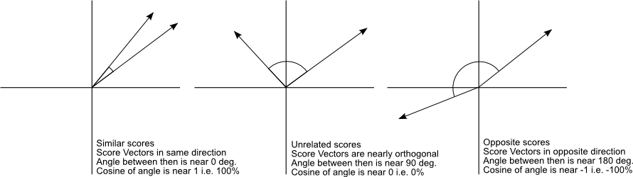
Image from a 2013 blog post by Christian S. Perone
For the data we’ll be looking at in this post, \(\text{cos}(\theta)\) will be somewhere between 0 and 1, since user play data is all non-negative. A value of 1 will indicate perfect similarity, and 0 will indicate the two vectors are unrelated. In other applications, there may be data which is positive and negative. For these cases, \(\text{cos}(\theta)\) will be between -1 and 1, with -1 meaning \(a\) and \(b\) are perfectly dissimilar and 1 meaning \(a\) and \(b\) are perfectly similar.
The Data: Songs from the Million Song Dataset
We use a subset of the data from the Million Song Dataset. The data only has 10K songs, but that should be enough for this exercise.
# read user play data and song data from the internet
play_data <- "https://static.turi.com/datasets/millionsong/10000.txt" %>%
  read_tsv(col_names = c('user', 'song_id', 'plays'))

song_data <- 'https://static.turi.com/datasets/millionsong/song_data.csv' %>%
  read_csv() %>%
  distinct(song_id, title, artist_name)
# join user and song data together
all_data <- play_data %>%
  group_by(user, song_id) %>%
  summarise(plays = sum(plays, na.rm = TRUE)) %>%
  inner_join(song_data)
Here are the first few rows of the data. The important variable is plays, which measures how many times a certain user has listened to a song. We’ll be using this variable to generate recommendations.
knitr::kable(head(all_data, 4))| user | song_id | plays | title | artist_name |
|---|---|---|---|---|
| 00003a4459f33b92906be11abe0e93efc423c0ff | SOJJRVI12A6D4FBE49 | 1 | Only You (Illuminate Album Version) | David Crowder*Band |
| 00003a4459f33b92906be11abe0e93efc423c0ff | SOKJWZB12A6D4F9487 | 4 | Do You Want To Know Love (Pray For Rain Album Version) | PFR |
| 00003a4459f33b92906be11abe0e93efc423c0ff | SOMZHIH12A8AE45D00 | 3 | You’re A Wolf (Album) | Sea Wolf |
| 00003a4459f33b92906be11abe0e93efc423c0ff | SONFEUF12AAF3B47E3 | 3 | Não É Proibido | Marisa Monte |
There are 76,353 users in this data set, so combining the number of users with songs makes the data a little too unwieldy for this toy example. I’m going to filter our dataset so that it’s only based on the 1,000 most-played songs. We use the spread function to turn our data from being “tall” (one row per user per song) to being “wide” (one row per user, and one column per song).
top_1k_songs <- all_data %>%
    group_by(song_id, title, artist_name) %>%
    summarise(sum_plays = sum(plays)) %>%
    ungroup() %>%
    top_n(1000, sum_plays) %>%
    distinct(song_id)

all_data_top_1k <- all_data %>%
  inner_join(top_1k_songs)

top_1k_wide <- all_data_top_1k %>%
    ungroup() %>%
    distinct(user, song_id, plays) %>%
    spread(song_id, plays, fill = 0)

ratings <- as.matrix(top_1k_wide[,-1])
This results in having play data for 70,345 users and 994 songs. 1.05% of user-song combinations have plays greater than 0.
Here’s a sample of what the ratings matrix looks like:
ratings[1:5, 1:3] # one row per user, one column per song## SOAAVUV12AB0186646 SOABHYV12A6D4F6D0F SOABJBU12A8C13F63F
## [1,] 0 0 0
## [2,] 0 0 0
## [3,] 0 0 0
## [4,] 0 0 0
## [5,] 0 0 0The Result: Making Song Recommendations
I wrote a function called calc_cos_sim, which will calculate the similarity between a chosen song and the other songs, and recommend 5 new songs for a user to listen to. From start to finish, this only took about 20 lines of code, indicating how easy it can be to spin up a recommendation engine.
calc_cos_sim <- function(song_code,
                         rating_mat = ratings,
                         songs = song_data,
                         return_n = 5) {
  # find our song
  song_col_index <- which(colnames(rating_mat) == song_code)
  # calculate cosine similarity for each song based on
  # number of plays for users
  # apply(..., 2) iterates over the columns of a matrix
  cos_sims <- apply(rating_mat, 2,
                    FUN = function(y)
                      cosine_sim(rating_mat[,song_col_index], y))
  # return results
  data_frame(song_id = names(cos_sims), cos_sim = cos_sims) %>%
    filter(song_id != song_code) %>% # remove self reference
    inner_join(songs) %>%
    arrange(desc(cos_sim)) %>%
    top_n(return_n, cos_sim) %>%
    select(song_id, title, artist_name, cos_sim)
}
We can use the function above to calculate similarities and generate recommendations for a few songs.
Let’s look at the hip-hop classic “Forgot about Dre” first.
forgot_about_dre <- 'SOPJLFV12A6701C797'
knitr::kable(calc_cos_sim(forgot_about_dre))| song_id | title | artist_name | cos_sim |
|---|---|---|---|
| SOZCWQA12A6701C798 | The Next Episode | Dr. Dre / Snoop Dogg | 0.3561683 |
| SOHEMBB12A6701E907 | Superman | Eminem / Dina Rae | 0.2507195 |
| SOWGXOP12A6701E93A | Without Me | Eminem | 0.1596885 |
| SOJTDUS12A6D4FBF0E | None Shall Pass (Main) | Aesop Rock | 0.1591929 |
| SOSKDTM12A6701C795 | What’s The Difference | Dr. Dre / Eminem / Alvin Joiner | 0.1390476 |
Each song we recommended is a hip-hop song, which is a good start! Even on this reduced dataset, the engine is making decent recommendations.
The next song is “Come As You Are” by Nirvana. Users who like this song probably listen to other grunge/rock songs.
come_as_you_are <- 'SODEOCO12A6701E922'
knitr::kable(calc_cos_sim(come_as_you_are))| song_id | title | artist_name | cos_sim |
|---|---|---|---|
| SOCPMIK12A6701E96D | The Man Who Sold The World | Nirvana | 0.3903533 |
| SONNNEH12AB01827DE | Lithium | Nirvana | 0.3568732 |
| SOLOFYI12A8C145F8D | Heart Shaped Box | Nirvana | 0.1958162 |
| SOVDLVT12A58A7B988 | Behind Blue Eyes | Limp Bizkit | 0.1186160 |
| SOWBYZF12A6D4F9424 | Fakty | Horkyze Slyze | 0.0952245 |
Alright, 2 for 2. One thing to be mindful of when looking at these results is that we’re not incorporating any information about the songs themselves. Our engine isn’t built using any data about the artist, genre, or other musical characteristics. Additionally, we’re not considering any demographic information about the users, and it’s fairly easy to see how useful age, gender, and other user-level data could be in making recommendations. If we used this information in addition to our user play data, we’d have what is called a hybrid recommendation system.
Finally, we’ll recommend songs for our hard-partying friends that like the song “Shots” by LMFAO featuring Lil Jon (that video is not for the faint of heart).
shots <- 'SOJYBJZ12AB01801D0'
knitr::kable(calc_cos_sim(shots))| song_id | title | artist_name | cos_sim |
|---|---|---|---|
| SOWEHOM12A6BD4E09E | 16 Candles | The Crests | 0.2551851 |
| SOLQXDJ12AB0182E47 | Yes | LMFAO | 0.1866648 |
| SOSZJFV12AB01878CB | Teach Me How To Dougie | California Swag District | 0.1387647 |
| SOYGKNI12AB0187E6E | All I Do Is Win (feat. T-Pain_ Ludacris_ Snoop Dogg & Rick Ross) | DJ Khaled | 0.1173063 |
| SOUSMXX12AB0185C24 | OMG | Usher featuring will.i.am | 0.1012716 |
Well, the “16 Candles” result is a little surprising, but this might give us some insight into the demographics of users that like “Shots”. The other four recommendations seem pretty solid, I guess.
Conclusion
Cosine similarity is simple to calculate and is fairly intuitive once some basic geometric concepts are understood. The simplicity of this metric makes it a great first-pass option for recommendation systems, and can be treated as a baseline with which to compare more computationally intensive and/or difficult to understand methods.
I think that recommendation systems will continue to play a large role in our online lives. It can be helpful to understand the components underneath these systems, so that we treat them less as blackbox oracles and more as the imperfect prediction systems based on data they are.
I hope you liked this brief excursion into the world of recommendation engines. Hopefully you can walk away knowing a little more about why Amazon, Netflix, and other platforms recommend the content they do.
Other Resources
Here are a few great resources if you want to dive deeper into recommendation systems and cosine similarity.
- Machine Learning :: Cosine Similarity for Vector Space Models (Part III)
- Series of blog posts about cosine similarity
- Wikipedia: Cosine Similarity
- Implementing and Understanding Cosine Similarity
- What are Product Recommendation Engines? And the various versions of them?
- Introduction to Collaborative Filtering