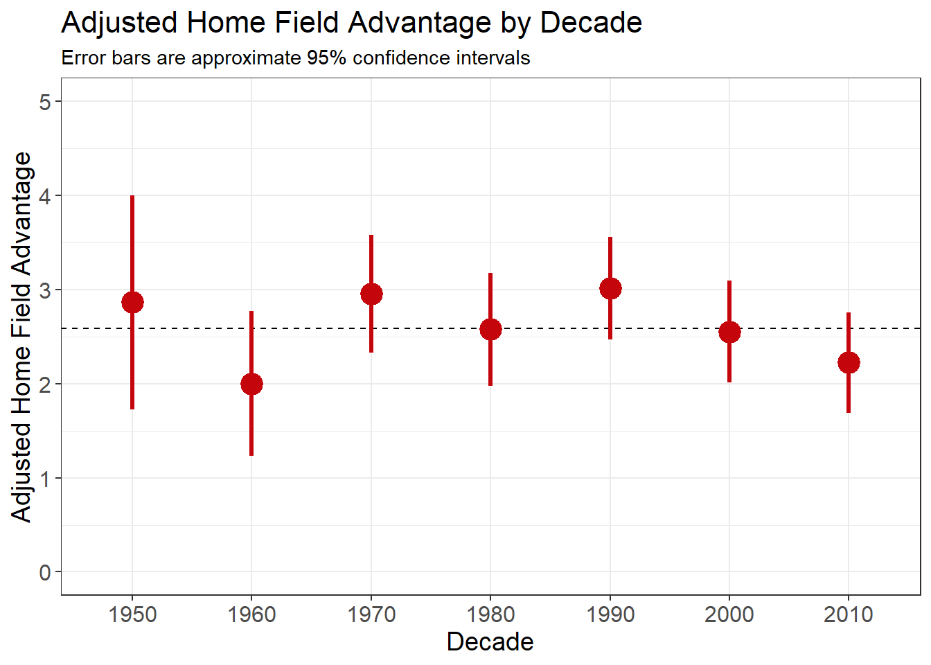
If you pay attention to NFL football, you’re probably used to hearing that homefield advantage is worth about 3 points. I’ve always been interested in this number, and how it was derived. So, using some data from FiveThirtyEight, along with some linear modeling in R, I attempted to quantify home field advantage. My analysis shows that home field advantage (how much we expect the home team to win by, if the teams are evenly matched) is about 2.59 points.
Here are the packages we’ll need:
library(tidyverse)
library(data.table)
library(ggridges)
library(scales)
You can find my code for this analysis on my GitHub.
Introduction
FiveThirtyEight has a data set with game-by-game Elo ratings and forecasts dating back to 1920. Elo ratings are simple measures of strength based on game-by-game results. More details on Elo ratings can be found here.
It’s pretty easy to get this data.
data_link <- "https://projects.fivethirtyeight.com/nfl-api/nfl_elo.csv"

nfl_data <- fread(data_link, verbose = FALSE)
Here are the first few rows and columns of the data:
| date | season | neutral | playoff | team1 | team2 | elo1_pre | elo2_pre |
|---|---|---|---|---|---|---|---|
| 1920-09-26 | 1920 | 0 | RII | STP | 1503.947 | 1300.000 | |
| 1920-10-03 | 1920 | 0 | DAY | COL | 1493.002 | 1504.908 | |
| 1920-10-03 | 1920 | 0 | RII | MUN | 1516.108 | 1478.004 | |
| 1920-10-03 | 1920 | 0 | CHI | MUT | 1368.333 | 1300.000 | |
| 1920-10-03 | 1920 | 0 | CBD | PTQ | 1504.688 | 1300.000 | |
| 1920-10-03 | 1920 | 0 | BFF | WBU | 1478.004 | 1300.000 |
The full description of the data can be found on FiveThirtyEight’s GitHub.
We’re interested in a few variables in this data:
| variable | definition |
|---|---|
| elo1_pre | Home team’s Elo rating before the game |
| elo2_pre | Away team’s Elo rating before the game |
| qbelo1_pre | Home team’s quarterback-adjusted base rating before the game |
| qbelo2_pre | Away team’s quarterback-adjusted base rating before the game |
| score1 | Home team’s score |
| score2 | Away team’s score |
To quantify home field advantage, we can look at the home vs away score differential for all games not played at a neutral site. We excluded playoff games from this analysis.
Here’s the summary of that score differential:
| measure | value |
|---|---|
| Min. | -57.00000 |
| 1st Qu. | -7.00000 |
| Median | 3.00000 |
| Mean | 2.59056 |
| 3rd Qu. | 12.00000 |
| Max. | 59.00000 |
The median margin of victory is 3. Since this number is positive, it implies that there is a noticeable home field advantage.
You might be wondering, has home field advantage been changing over time?
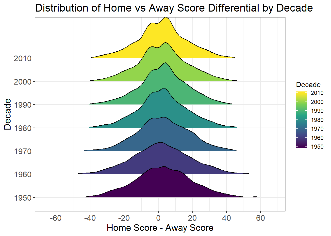
If you look at the most recent decades, you’ll notice that the distribution has been becoming bimodal, meaning there are two “peaks” in the distribution. The peaks belong to margins of victory of three points (a field goal) for the home and away teams:
| Decade | Home - Away | Count of Games | % of Games |
|---|---|---|---|
| 2010 | 3 | 203 | 8.02% |
| 2010 | -3 | 165 | 6.52% |
| 2000 | 3 | 225 | 8.87% |
| 2000 | -3 | 173 | 6.82% |
| 1990 | 3 | 196 | 8.419% |
| 1990 | -3 | 181 | 7.775% |
| 1980 | 3 | 159 | 7.472% |
| 1980 | -3 | 139 | 6.532% |
| 1970 | 3 | 102 | 5.280% |
| 1970 | -3 | 98 | 5.072% |
| 1960 | 3 | 84 | 5.214% |
| 1960 | 0 | 72 | 4.469% |
| 1950 | 3 | 37 | 5.096% |
| 1950 | -4 | 35 | 4.821% |
It’s not just good enough to take the average or median of all home vs away score differentials. Each NFL game is different, and by just blindly taking a summary statistic, we are assuming that the teams playing in each game are evenly matched. In my opinion, this assumption is invalid.
We can use linear models to get closer to understanding home field advantage, by adjusting for the differences between the two teams. But before we get too deep into that, let’s take a closer look at linear regression.
Linear Regression Basics
A lot of people are familiar with linear models, having performed “line of best fit” calculations sometime in high school. Most people cringe when they see the \(y = mx + b\) formula, but statisticians and data scientists feel their hearts warm and get very excited after glancing at that formula.
Linear models are incredibly powerful tools of statistical analysis. Most of the time, we spend a lot of energy interpreting the \(m\) in the equation above. This gives us insight into how much we expect \(y\) to change (on average) when \(x\) changes by some amount.
To illustrate, let’s use the mtcars data set to predict a car’s miles per gallon using its weight in pounds.
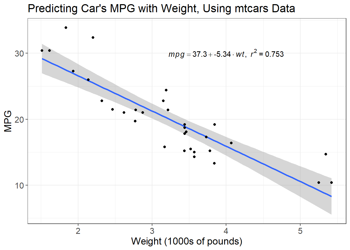
The linear model’s formula is displayed in the upper right hand corner of the plot. The coefficient for \(wt\) is -5.3, this is the \(m\) in the \(y = mx + b\) equation. The coefficient is negative, meaning that as the weight of the car increases, we expect its fuel efficiency to get worse. But what about \(b\), the intercept of the line?
The intercept of the best fit line is our “predicted” value of \(y\) when \(x\) equals 0. So, when the weight of a car is 0 pounds, we expect it to get 37.29 miles per gallon. This doesn’t make any sense! A car that weighs 0 pounds doesn’t get any miles per gallon, it doesn’t even exist!
In a lot of linear models, the intercept isn’t really worth interpreting. However, we can use the intercept to understand home field advantage using our NFL data.
Interpreting the Intercept in a Model of the NFL
We first fit a model trying to predict the home vs away score differential using the home vs away pre game Elo differential and the home vs away pre game QB Elo differential.
When the Elo differentials are equal to zero, it means the teams are effectively even matched (our best guess for the power rankings of the respective teams are basically equal). This gets us closer to understanding true home field advantage than taking a summary statistic would.
Our model will look like:
\[ \text{Home - Away Score} = \beta_{0} + \beta_{1} *\text{Elo Difference} + \beta_{2} * \text{QB Elo Difference}\]
While \(\beta_{1}\) and \(\beta_{2}\) above are interesting, we’re most interested in \(\beta_{0}\), since this quantifies the home field advantage for evenly matched teams.
Enough talking, let’s fit the model:
score_diff_model <- lm(home_away_score_diff ~ home_away_elo_diff+home_away_qb_elo_diff,
data = model_data)| term | estimate |
|---|---|
| (Intercept) | 2.586 |
| home_away_elo_diff | 0.037 |
| home_away_qb_elo_diff | 0.021 |
Touchdown!
If we look at the intercept, the value is about 2.59. This means that if the two teams are basically evenly matched (i.e. \(x=0\) in \(y = mx+b\)), we can expect the home team to win by about 2.59 points (on average).
Taking it one step further, here are the home field advantages for each decade.
Wrapping Up
We can learn some pretty cool things about our data if we pay close attention to the output of our linear models. I think a lot of people forget to pay attention to the intercepts in their linear models. This makes sense most of the time, because the intercept doesn’t really mean much in many of our models (e.g. if we predict a person’s height using their weight, the intercept is meaningless).
However, in some cases the intercept is really important. In this example using NFL data, we were able to use the intercept to quantify home field advantage for evenly matched teams. Hopefully this post will give a data point to bring up at a nice dinner party where you and your acquaintances are discussing what home field advantage really means.