This post was originally meant for the R Users Group at my organization. I thought it would be worthwhile to have it on my blog as well, in case anyone out there is searching for a short introduction to the data.table package.
Although the primary data wrangling package I use is tidyverse, it’s worthwhile to explore other packages that do similar data manipulations. The closest “competitor” to the tidyverse is the data.table package.

Data Wrangling
Three of the main selling points for using data.table are that it’s
- Fast
- Concise
- We’ll go through a few examples using the
data.tablesyntax
- We’ll go through a few examples using the
- Efficient
- Works well with large data
These are three qualities we look for in data manipulation.
If you’re frustrated by how verbose data manipulation chains can get using tidyverse packages, data.table might be right for you.
Here are the packages we’ll need for this post.
library(data.table)
library(nycflights13)
library(microbenchmark)
library(tidyverse)
The data set we’ll be working with in this post comes from the nycflights13 package. It shows on-time data for all flights that departed NYC in 2013.
(flights_dt <- as.data.table(flights)) # convert to a data.table## year month day dep_time sched_dep_time dep_delay arr_time
## 1: 2013 1 1 517 515 2 830
## 2: 2013 1 1 533 529 4 850
## ---
## 336775: 2013 9 30 NA 1159 NA NA
## 336776: 2013 9 30 NA 840 NA NA
## sched_arr_time arr_delay carrier flight tailnum origin dest air_time
## 1: 819 11 UA 1545 N14228 EWR IAH 227
## 2: 830 20 UA 1714 N24211 LGA IAH 227
## ---
## 336775: 1344 NA MQ 3572 N511MQ LGA CLE NA
## 336776: 1020 NA MQ 3531 N839MQ LGA RDU NA
## distance hour minute time_hour
## 1: 1400 5 15 2013-01-01 05:00:00
## 2: 1416 5 29 2013-01-01 05:00:00
## ---
## 336775: 419 11 59 2013-09-30 11:00:00
## 336776: 431 8 40 2013-09-30 08:00:00paste(dim(flights_dt), c("rows", "columns"))## [1] "336776 rows" "19 columns"Demo
The basics
If you’re familiar with SQL, data.table syntax should make a good amount of sense. The syntax allows you to do a lot more than the common operations we expect with a base data.frame. Here is the general form of data.table syntax:
DT[i, j, by]i: where (subset) / order by (sort)j: select (grab certain columns) / update (add/modify columns)by: group by
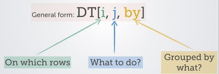
Image source: Blazing Fast Data Wrangling With R data.table
To demonstrate, let’s take a look at each of these components.
Subset and sort with i
The first three examples look at using i to filter/subset your data.
# flights departing in January
flights_dt[month == 1]
## year month day dep_time sched_dep_time dep_delay arr_time sched_arr_time
## 1: 2013 1 1 517 515 2 830 819
## 2: 2013 1 1 533 529 4 850 830
## ---
## 27003: 2013 1 31 NA 1446 NA NA 1757
## 27004: 2013 1 31 NA 625 NA NA 934
## arr_delay carrier flight tailnum origin dest air_time distance hour
## 1: 11 UA 1545 N14228 EWR IAH 227 1400 5
## 2: 20 UA 1714 N24211 LGA IAH 227 1416 5
## ---
## 27003: NA UA 337 <NA> LGA IAH NA 1416 14
## 27004: NA UA 1497 <NA> LGA IAH NA 1416 6
## minute time_hour
## 1: 15 2013-01-01 05:00:00
## 2: 29 2013-01-01 05:00:00
## ---
## 27003: 46 2013-01-31 14:00:00
## 27004: 25 2013-01-31 06:00:00# flights departing on March 10th
flights_dt[month == 3 & day == 10]## year month day dep_time sched_dep_time dep_delay arr_time sched_arr_time
## 1: 2013 3 10 6 2359 7 336 338
## 2: 2013 3 10 41 2100 221 230 2257
## ---
## 907: 2013 3 10 NA 2000 NA NA 2335
## 908: 2013 3 10 NA 1730 NA NA 1923
## arr_delay carrier flight tailnum origin dest air_time distance hour minute
## 1: -2 B6 727 N547JB JFK BQN 186 1576 23 59
## 2: 213 EV 4368 N14116 EWR DAY 82 533 21 0
## ---
## 907: NA UA 424 <NA> EWR SAT NA 1569 20 0
## 908: NA US 449 <NA> EWR CLT NA 529 17 30
## time_hour
## 1: 2013-03-10 23:00:00
## 2: 2013-03-10 21:00:00
## ---
## 907: 2013-03-10 20:00:00
## 908: 2013-03-10 17:00:00# flights where the total delay (dep_delay + arr_delay) is 10 minutes or more,
# the destination was Dallas (DFW) and was in January, February, or March
flights_dt[(dep_delay + arr_delay) >= 10 & dest == "DFW" & month <= 3]## year month day dep_time sched_dep_time dep_delay arr_time sched_arr_time
## 1: 2013 1 1 559 600 -1 941 910
## 2: 2013 1 1 635 635 0 1028 940
## ---
## 574: 2013 3 31 1308 1300 8 1622 1605
## 575: 2013 3 31 1923 1825 58 2202 2127
## arr_delay carrier flight tailnum origin dest air_time distance hour minute
## 1: 31 AA 707 N3DUAA LGA DFW 257 1389 6 0
## 2: 48 AA 711 N3GKAA LGA DFW 248 1389 6 35
## ---
## 574: 17 AA 745 N3CAAA LGA DFW 218 1389 13 0
## 575: 35 UA 1221 N35271 EWR DFW 196 1372 18 25
## time_hour
## 1: 2013-01-01 06:00:00
## 2: 2013-01-01 06:00:00
## ---
## 574: 2013-03-31 13:00:00
## 575: 2013-03-31 18:00:00We can also sort using i:
# sort by total delay
flights_dt[order(dep_delay + arr_delay, decreasing = T)]
## year month day dep_time sched_dep_time dep_delay arr_time
## 1: 2013 1 9 641 900 1301 1242
## 2: 2013 6 15 1432 1935 1137 1607
## ---
## 336775: 2013 9 30 NA 1159 NA NA
## 336776: 2013 9 30 NA 840 NA NA
## sched_arr_time arr_delay carrier flight tailnum origin dest air_time
## 1: 1530 1272 HA 51 N384HA JFK HNL 640
## 2: 2120 1127 MQ 3535 N504MQ JFK CMH 74
## ---
## 336775: 1344 NA MQ 3572 N511MQ LGA CLE NA
## 336776: 1020 NA MQ 3531 N839MQ LGA RDU NA
## distance hour minute time_hour
## 1: 4983 9 0 2013-01-09 09:00:00
## 2: 483 19 35 2013-06-15 19:00:00
## ---
## 336775: 419 11 59 2013-09-30 11:00:00
## 336776: 431 8 40 2013-09-30 08:00:00Select and create new columns using j
This first example shows how to select a column. It looks very similar to what we’d do in base R.
# get flight destination
destination <- flights_dt[, dest]
head(destination)
## [1] "IAH" "IAH" "MIA" "BQN" "ATL" "ORD"You’ll notice that the result of the previous operation was a vector. Sometimes this is what we want, other times it’s not. So, how can we select a column and have a data.table returned instead of a vector?
We can use .(column_I_want, another_column_I_want) or list(this_column_too, and_this_one_also).
# use .(columns_to_select) or list(columns_to_select)
# .(columns_to_select) acts as "shorthand" for list(columns_to_select)
flights_dt[,.(dest)]
## dest
## 1: IAH
## 2: IAH
## ---
## 336775: CLE
## 336776: RDU# we can select multiple columns using .()
flights_dt[,.(year, month, day, origin, dest)]## year month day origin dest
## 1: 2013 1 1 EWR IAH
## 2: 2013 1 1 LGA IAH
## ---
## 336775: 2013 9 30 LGA CLE
## 336776: 2013 9 30 LGA RDU# rename columns
flights_dt[,.(Origin = origin, Destination = dest)]## Origin Destination
## 1: EWR IAH
## 2: LGA IAH
## ---
## 336775: LGA CLE
## 336776: LGA RDUWe can create columns using :=:
# create total delay column
flights_dt[,total_delay := arr_delay + dep_delay]
One major difference between “standard” operations in R and some operations in data.table is that data.table will make modifications in place, meaning we don’t have to use the assignment operator (<- or =).
If we inspect flights_dt, we can confirm that the total_delay column was added.
flights_dt## year month day dep_time sched_dep_time dep_delay arr_time
## 1: 2013 1 1 517 515 2 830
## 2: 2013 1 1 533 529 4 850
## ---
## 336775: 2013 9 30 NA 1159 NA NA
## 336776: 2013 9 30 NA 840 NA NA
## sched_arr_time arr_delay carrier flight tailnum origin dest air_time
## 1: 819 11 UA 1545 N14228 EWR IAH 227
## 2: 830 20 UA 1714 N24211 LGA IAH 227
## ---
## 336775: 1344 NA MQ 3572 N511MQ LGA CLE NA
## 336776: 1020 NA MQ 3531 N839MQ LGA RDU NA
## distance hour minute time_hour total_delay
## 1: 1400 5 15 2013-01-01 05:00:00 13
## 2: 1416 5 29 2013-01-01 05:00:00 24
## ---
## 336775: 419 11 59 2013-09-30 11:00:00 NA
## 336776: 431 8 40 2013-09-30 08:00:00 NAWe can remove a column by setting it := to NULL.
# remove that column
flights_dt[,total_delay:=NULL]
flights_dt
## year month day dep_time sched_dep_time dep_delay arr_time
## 1: 2013 1 1 517 515 2 830
## 2: 2013 1 1 533 529 4 850
## ---
## 336775: 2013 9 30 NA 1159 NA NA
## 336776: 2013 9 30 NA 840 NA NA
## sched_arr_time arr_delay carrier flight tailnum origin dest air_time
## 1: 819 11 UA 1545 N14228 EWR IAH 227
## 2: 830 20 UA 1714 N24211 LGA IAH 227
## ---
## 336775: 1344 NA MQ 3572 N511MQ LGA CLE NA
## 336776: 1020 NA MQ 3531 N839MQ LGA RDU NA
## distance hour minute time_hour
## 1: 1400 5 15 2013-01-01 05:00:00
## 2: 1416 5 29 2013-01-01 05:00:00
## ---
## 336775: 419 11 59 2013-09-30 11:00:00
## 336776: 431 8 40 2013-09-30 08:00:00# add multiple columns
flights_dt[, `:=`(date = lubridate::ymd(paste(year, month, day, sep = "-")),
log_distance = log(distance),
air_time_in_hours = air_time / 60)]
flights_dt## year month day dep_time sched_dep_time dep_delay arr_time
## 1: 2013 1 1 517 515 2 830
## 2: 2013 1 1 533 529 4 850
## ---
## 336775: 2013 9 30 NA 1159 NA NA
## 336776: 2013 9 30 NA 840 NA NA
## sched_arr_time arr_delay carrier flight tailnum origin dest air_time
## 1: 819 11 UA 1545 N14228 EWR IAH 227
## 2: 830 20 UA 1714 N24211 LGA IAH 227
## ---
## 336775: 1344 NA MQ 3572 N511MQ LGA CLE NA
## 336776: 1020 NA MQ 3531 N839MQ LGA RDU NA
## distance hour minute time_hour date log_distance
## 1: 1400 5 15 2013-01-01 05:00:00 2013-01-01 7.244228
## 2: 1416 5 29 2013-01-01 05:00:00 2013-01-01 7.255591
## ---
## 336775: 419 11 59 2013-09-30 11:00:00 2013-09-30 6.037871
## 336776: 431 8 40 2013-09-30 08:00:00 2013-09-30 6.066108
## air_time_in_hours
## 1: 3.783333
## 2: 3.783333
## ---
## 336775: NA
## 336776: NAGrouping with by
In the first two examples, we use .N, which is a special symbol which allows us to count rows in our data. .SD, which is used later on in this post, is also a special symbol in data.table.
A simple example, counting by origin of flight.
flights_dt[,.N,origin]## origin N
## 1: EWR 120835
## 2: LGA 104662
## 3: JFK 111279A little more complicated, counting by origin and destination, then sorting to show most frequent, then slice top 10 rows.
flights_dt[,.N, .(origin, dest)][order(-N)][1:10]## origin dest N
## 1: JFK LAX 11262
## 2: LGA ATL 10263
## 3: LGA ORD 8857
## 4: JFK SFO 8204
## 5: LGA CLT 6168
## 6: EWR ORD 6100
## 7: JFK BOS 5898
## 8: LGA MIA 5781
## 9: JFK MCO 5464
## 10: EWR BOS 5327To wrap up this section, let’s show the median and average total delay by origin and destination airport, and then sort by average total delay. We also add in .N, because it’s always good to show the sample size.
flights_dt[!is.na(arr_delay) & !is.na(dep_delay),
           .(avg_delay = mean(arr_delay + dep_delay),
             median_delay = median(arr_delay + dep_delay),
             .N),
           .(origin, dest)
           ][order(-avg_delay)]
## origin dest avg_delay median_delay N
## 1: EWR TYS 82.80511 18 313
## 2: EWR CAE 78.94681 40 94
## ---
## 222: JFK PSP -15.66667 -14 18
## 223: LGA LEX -31.00000 -31 1A little more advanced

Turning it up
We often want to perform multiple operations on a single data.frame. If we keep all of the code to perform these operations on a single line, our scripts can become illegible and unwieldy. Similar to how tidyverse pipes might span multiple lines:
data %>%
  mutate(new_columns) %>%
  group_by(grouping_columns) %>%
  summarise(other_columns) %>%
  arrange(desc(some_column))
We can “chain” data.table expressions:
DT[ ...
   ][ ...
     ][ ...
       ]
This example gets the cumulative total delay over the course of a year by origin airport. It utilizes filtering, sorting, and grouping.
# get cumulative delay by origin airport
# uses "chaining"
cumulative_delay_by_origin <-
  flights_dt[!is.na(dep_delay) & !is.na(arr_delay) # keep valid flights
             ][order(time_hour),                   # sort by date
               .(time_hour,                        # select date and cumsum delay
                 cumu_delay=cumsum(arr_delay+dep_delay)),
               origin]                             # group by origin airport

ggplot(cumulative_delay_by_origin,
       aes(time_hour, cumu_delay/60, colour = origin))+
  geom_line()+
  theme_bw()+
  xlab("Date") + ylab("Cumulative total delay (hours)")
Let’s get even crazier with chaining.
The next example finds the “biggest loser” on each day (i.e. which flight had the worst total delay). We then count up (using the ones column) which origin airport the biggest loser was departing from. We calculate this cumulatively over the course of the year.
top_delay <- flights_dt[!is.na(arr_delay) & !is.na(dep_delay)
                        ][,`:=`(total_delay=arr_delay+dep_delay, ones=1)
                          ][, .SD[ which.max(total_delay) ], date
                            ][order(date)
                              ][,.(cumu_obs = cumsum(ones), date),.(origin)]

ggplot(top_delay, aes(date, cumu_obs, colour = origin))+
  geom_line()+
  theme_bw()+
  xlab("Date")+
  ylab("Cumulative # of Days with Worst Delay")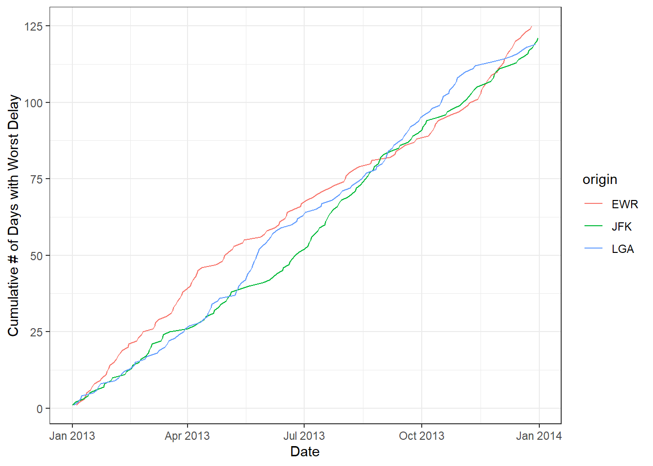
Performance evaluation: base R, tidyverse, and data.table
Let’s demonstrate a typical calculation you might do in R: an aggregation of two columns based on grouping by three columns. In this specific example, we’re calculating the average departure delay and average arrival delay by origin airport, destination airport, and month of flight.
We use the microbenchmark package to time how long it takes to perform the different operations. We can then take the results and visualize them.
set.seed(1848)
benchmark_data <- microbenchmark(
  # base R solution
  base_R = aggregate(list(flights$dep_delay, flights$arr_delay),
                     list(flights$origin, flights$dest, flights$month),
                     mean, na.rm = TRUE),
  # tidyverse solution
  tidy_verse = flights %>%
    group_by(origin, dest, month) %>%
    summarise_at(c("dep_delay", "arr_delay"), mean, na.rm = TRUE),

  #data.table
  data_table = flights_dt[,lapply(.SD, mean, na.rm = TRUE),
                          .(origin, dest, month),
                          .SDcols = c("dep_delay", "arr_delay")],

  times = 100)
library(ggridges)
benchmark_data_dt <- as.data.table(benchmark_data)
benchmark_data_dt[,time_in_ms := time / 1000000]
ggplot(benchmark_data_dt, aes(x = time_in_ms, y = expr))+
geom_density_ridges2(rel_min_height = 0.01, scale = 1.5, fill = "#c5050c")+
geom_boxplot(width = 0.25)+
theme_bw()+
scale_x_log10("Time (milliseconds, log10)")+
scale_y_discrete("Operation",
labels = c("base_R" = "Base R",
"tidy_verse" = "tidyverse",
"data_table" = "data.table"))+
ggtitle("Grouped Aggregation Timing Summary")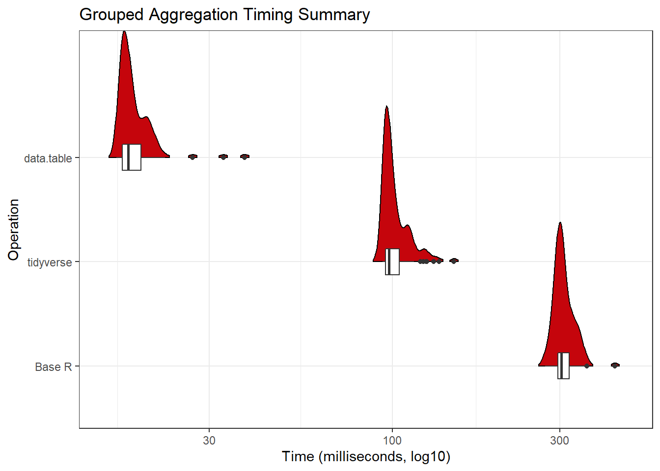
Here is how much slower the median operation is compared to data.table. Since this is a tutorial about data.table, we use its dcast function to convert long data to wide.
dcast(benchmark_data_dt,
      .~expr,
      value.var = "time_in_ms",
      fun = median)[, round(.SD/data_table,1),
                    .SDcols = c("base_R", "tidy_verse", "data_table")]
## base_R tidy_verse data_table
## 1: 17.2 5.5 1The short demo above demonstrates just how much more performant using data.table can be.
Here’s a more complete reference on benchmarking, with comparisons across R and Python.
Summary
I hope this was a gentle introduction to the data.table package. I think the key to getting off on the right foot with this package is understanding the syntax.
The syntax allows you to do a lot more than the common operations we expect with a base data.frame. Here is the general form of data.table syntax:
DT[i, j, by]i: where (subset) / order by (sort)j: select (grab certain columns) / update (add/modify columns)by: group by
Image source: Blazing Fast Data Wrangling With R data.table
By no means did I intend for this introduction to be an exhaustive guide to all things data.table. If you’re interested in exploring the package further, take a look at these resources:
Postscript: Fun fact
Fun R fact: <- and = are actually functions, and can be called like so:
`<-`(x, 1:5)
x
## [1] 1 2 3 4 5`=`(x, 5:1)
x## [1] 5 4 3 2 1`<-`(x, c(rev(x), x))
x## [1] 1 2 3 4 5 5 4 3 2 1`<-`("ill-advised variable name", 1:3)
`ill-advised variable name`## [1] 1 2 3`=`("Christopher Guest Movies", "awesome")
`Christopher Guest Movies`## [1] "awesome"